

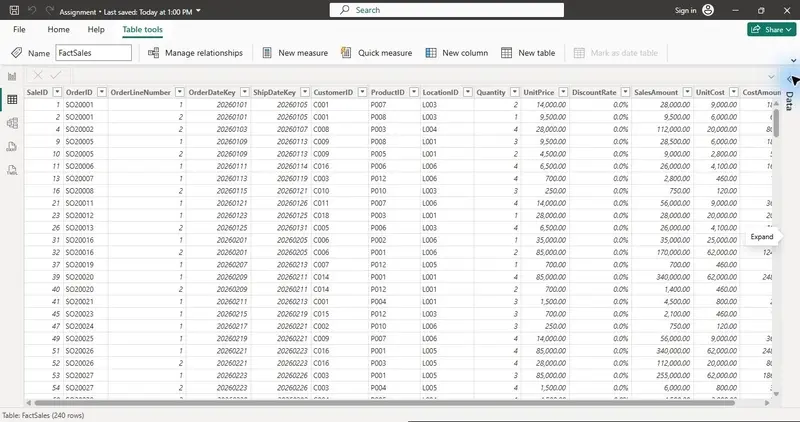
Executive Overview
In the modern enterprise landscape, Business Intelligence (BI) platforms are only as powerful as the data models that underpin them. As organizations aggregate data from a disparate array of sources—including legacy SQL databases, cloud platforms, flat Excel files, and third-party APIs—the necessity for structured, logically sound data architecture becomes paramount. Power BI relies heavily on a foundational understanding of how disparate tables interact to provide accurate answers to complex analytical queries.
Data modelling in Power BI involves much more than simply dragging and dropping tables together; it is a deliberate architectural discipline. It dictates how filters propagate through a system, how business data is represented for deep analysis, and how efficiently queries execute at scale. While flat tables offer an invitingly simple starting point for small datasets, they quickly degrade in performance and maintainability as transaction volumes grow. Conversely, advanced normalized models like snowflake schemas introduce unnecessary complexity. For the vast majority of enterprise implementations, the star schema emerges as the gold standard—delivering an optimal balance between query performance, model scalability, and maintainability.

Detailed Chronology & Conceptual Evolution
To understand the evolution of data modeling in Power BI, one must examine the progression from rudimentary data storage techniques to sophisticated analytical frameworks.
The Flat Table Model: Simplicity at a Cost
Historically, early reporting began with the flat table model, where all information—transactions, customer data, product attributes, and calendar dates—resides within a single, wide structure. For instance, a retail table might combine OrderID, Customer, County, Product, Category, Quantity, and SalesAmount into one grid.

- The Advantages: Flat tables eliminate the need for relationships. Visualizations can reference columns directly from a single data source, making it ideal for quick, exploratory ad-hoc analysis on small datasets.
- The Disadvantages: The architectural flaw is data repetition. If a single customer executes 10,000 transactions, their name and geographic location are replicated 10,000 times. This bloats file sizes, degrades compression efficiency, and makes it difficult to separate descriptive attributes from measurable business events.
The Star Schema Paradigm
Recognizing the limitations of flat tables, data architects developed the star schema. A star schema features a central fact table surrounded by a constellation of dimension tables. The central fact table houses measurable business events (such as sales amounts or quantities sold), while the surrounding dimensions contain descriptive attributes (such as customer segments, product categories, and calendar dates).
flowchart TB
    CUSTOMER["DimCustomer<br/>CustomerID<br/>CustomerName<br/>Segment"]
    PRODUCT["DimProduct<br/>ProductID<br/>ProductName<br/>Category"]
    DATE["DimDate<br/>DateKey<br/>Date<br/>Month<br/>Year"]
    LOCATION["DimLocation<br/>LocationID<br/>County<br/>Region"]

    SALES["FactSales<br/>SaleID<br/>CustomerID<br/>ProductID<br/>DateKey<br/>LocationID<br/>Quantity<br/>SalesAmount"]

    CUSTOMER --> SALES
    PRODUCT --> SALES
    DATE --> SALES
    LOCATION --> SALES
This structural separation ensures that descriptive data is stored once and reused efficiently, allowing Power BI’s VertiPaq engine to compress columns and accelerate query performance.

The Snowflake Schema: Deep Normalization
A snowflake schema extends the star schema by further normalizing dimension tables into sub-dimensions. For example, instead of storing product categories directly within the DimProduct table, categories are broken out into a separate DimCategory table linked by a foreign key.
While this eliminates redundancy within dimensions and naturally handles complex, reusable hierarchies, it comes with architectural trade-offs. The proliferation of additional tables and relationships increases model complexity and can hinder query performance in Power BI due to longer filter paths.

Supporting Context & Metrics: Dimensions vs. Facts
At the heart of dimensional modeling lies the strict separation of facts and dimensions. A simple heuristic for architects is to ask directional questions of the data elements:
- Dimensions describe: Who? What? Where? When? (e.g., Customer Name, Product Category, County, Month)
- Facts measure: How many? How much? How long? How often? (e.g., Quantity, Revenue, Profit, Cost)
Grain and Granularity
The grain of a fact table defines precisely what a single row represents. This must be established during the initial design phase. For instance, if an order ORD1001 contains three distinct items, a well-structured fact table will contain three rows—one for each product line on the transaction—rather than one row per order.

$$textGrain = textOne row per product per transaction line$$
Mixing different grains within a single fact table leads to corrupted aggregations and inaccurate reporting. Microsoft’s official modeling guidance explicitly mandates maintaining a consistent grain across all fact tables.

Primary and Foreign Keys
Relationships depend on the interaction between primary and foreign keys:
- Primary Keys: Uniquely identify each record within a dimension table (e.g., a unique
CustomerIDinDimCustomer). - Foreign Keys: Reference the corresponding primary key in the fact table, allowing the same key to appear multiple times as a customer makes recurring purchases.
Architectural Mechanisms: Relationships, Cardinality, and Filtering
Configuring the semantic model correctly requires careful attention to cardinality and filter propagation.

Cardinality Types
- *One-to-Many (1:):** The bedrock of a star schema. One row on the dimension side relates to many rows in the fact table. This should be the dominant pattern in your model.
- One-to-One (1:1): Each key occurs only once in both tables. This often indicates that the two tables should be combined, though it is occasionally used to segregate security profiles or sensitive employee data.
- Many-to-Many (*:*): Occurs when multiple rows on one side relate to multiple rows on the other (e.g., students and courses). In relational modelling, this is resolved using a bridge table to convert the structure into two clean 1:* relationships.
Filter Direction: Single vs. Bidirectional
Relationships do more than just connect tables; they dictate how filters move through the model.
- Single-Direction Filtering: Filters flow from the
1side (dimensions) to the*side (facts). This ensures predictable filter behavior, high query performance, and intuitive DAX calculations. - Bidirectional Filtering: Allows filters to propagate both ways. While useful for specific edge cases (such as security role-playing or specialized calculations), excessive bidirectional filtering introduces ambiguous filter paths, degrades performance, and creates unexpected reporting results. Microsoft recommends minimizing its use.
Power Query Merging vs. Semantic Model Relationships
A frequent point of confusion for developers is determining when to combine data via Power Query (merging) versus relating tables in the semantic model.

| Feature | Power Query Merge | Power BI Relationship |
|---|---|---|
| Stage | Data Preparation / Transformation | Semantic Model Configuration |
| Storage | Physically combines columns into a single table | Keeps tables separate; connects via logical links |
| Redundancy | High (repeats descriptive data across rows) | Low (maintains normalized dimensions) |
| Flexibility | Static transformation | Dynamic context filtering |
When to Merge
Merge data in Power Query when two datasets logically need to become a single query during ingestion—such as attaching exchange-rate lookup data to transactions, combining subsidiary employee attributes, or performing data-quality validation using anti-joins.
When to Relate
Relate tables within the semantic model when they represent distinct analytical entities (such as customers, products, dates, and sales events). Flattening a star schema into a single mega-table via excessive merging destroys the analytical integrity of the model, introduces massive data redundancy, and complicates DAX measure writing.

Future Outlook & Recommended Design Principles
As data volumes continue to expand exponentially, enterprise analytics solutions must be built for resilience, scalability, and performance. Adhering to proven architectural principles ensures that Power BI environments remain performant and maintainable over time.
Key Architectural Takeaways:
- Prioritize the Star Schema: Always default to a star schema design to leverage the full compression and performance capabilities of the VertiPaq engine.
- Maintain a Consistent Grain: Ensure that all fact tables maintain a uniform level of granularity to prevent aggregation errors.
- Enforce Single-Direction Relationships: Design your filter paths to flow cleanly from dimensions to fact tables, reserving bidirectional filters strictly for verified edge cases.
- Isolate Transformations: Perform structural joins and data cleansing in Power Query, reserving semantic relationships for the data model.
- Design Before You Build: Establish your schema, keys, grain, and relationships before writing complex DAX measures or designing user-facing dashboards.
By grounding your Power BI development in these robust data-modelling foundations, you ensure that your analytics remain performant, scalable, and trusted across the entire enterprise.